Getting Started with Jupyter Notebook

Jupyter Notebook is a popular IDE (Integrated Development Environment) that is known for its ease of use, and it’s unique features to contain both code and rich text elements, such as figures, links, equations. Due to this unique feature, the documents produced with Jupyter Notebook are the ideal place to bring together an analysis description, and its results as well as they can be executed to perform data analysis in real-time. A combination of the features listed above, as well as the ease of shareability of the “Notebooks” has made Jupyter Notebook a popular choice amongst Data Scientists and Data Engineers.

Installation

The easiest way to install Jupyter Notebook is by installing Anaconda (a popular Data Science Platform) from here. The installation of Anaconda is straightforward, but please ensure that the right installer for your operating system is downloaded.

Using Anaconda

After completing the Anaconda installation, you should have access to the following:

• Anaconda Navigator
• Anaconda Prompt

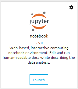
Anaconda Navigator uses the Graphical User-Interface to allow users to launch and manage (Install and Delete) tools that are packaged by Anaconda. It is very easy to navigate to the tools that you need using this dashboard. Currently, you only need to “Launch” Jupyter Notebook:

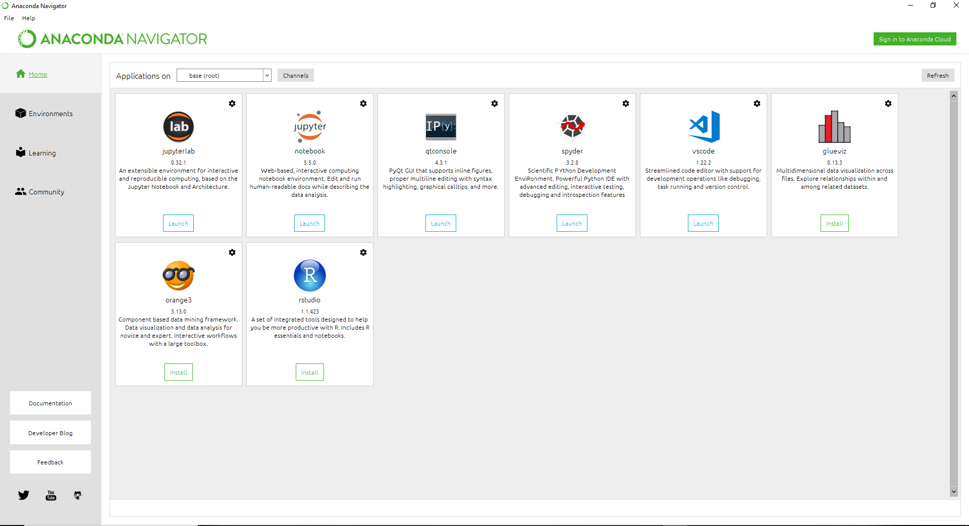
This can be achieved by clicking on the following Launch button.

The other way to Launch Jupyter Notebook is through the use of Anaconda’s command prompt. This is a preferable way of using this application as you have more control over the configuration and directory in which you want the Jupyter Notebook to be opened.

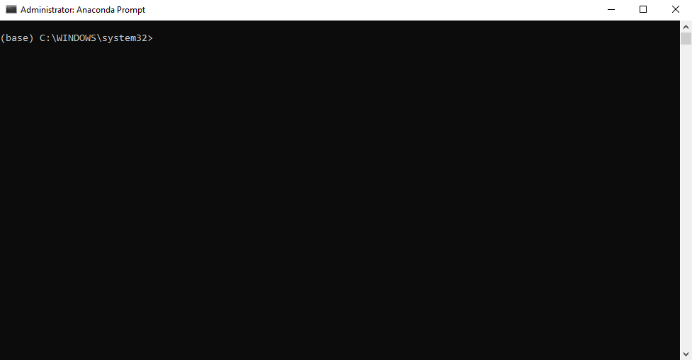
To get started with “Anaconda Command Prompt”, search for it in the Start Menu (for Windows users) and run it as Administrator. The following screen should appear.

It’s favourable to create a directory in the location you want to start your Jupyter Notebook projects. After successfully creating your directory, type the following in the command-line:

cd [Directory Location and Name]

jupyter notebook

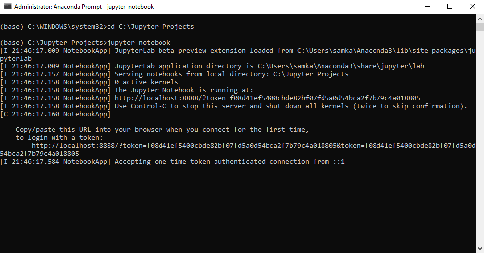
Typing “jupyter notebook” will start the application on port 8888 by default and opens the Jupyter Notebook in your default Web Browser. If you close the Prompt it will stop the server and kernel(s).

Jupyter Notebook runs in a browser and has a very simple yet powerful GUI.

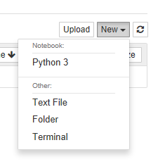
To demonstrate the real power of Jupyter Notebook, run some simple Python code. In this example, we will try to keep the use of libraries to a minimum. To get started, click on the “New” icon on the upper right side of the screen. Doing so will open a drop-down with a list of actions it can perform. Additional options, such as Kernels for Python 2 or R, may appear depending on your installation.

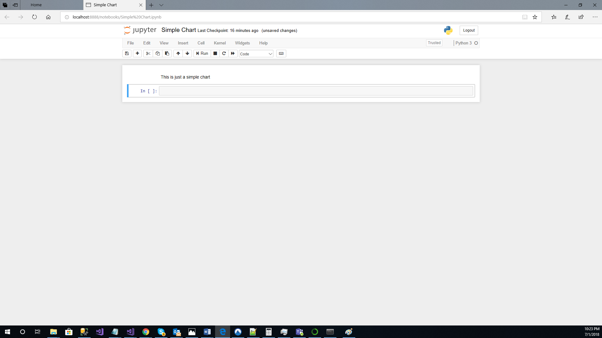
For demonstration purposes, let’s launch a “Python 3” notebook. Doing so will open a new tab that is using “Python 3” kernel. The page name is Untitled by default. To give it a name click on “Untitled”, and change Untitled to “Simple Chart” by typing the new name in the popup window’s text-field and clicking on “Rename” button.

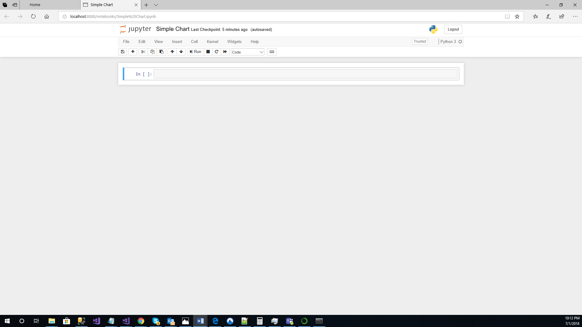
The name is changed successfully.

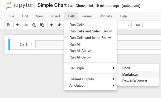
The above “Cell” is where your code and pictures etc. go. To write some texts, in the command bar click on “Cell” -> “Cell Type” -> “Markdown”. Doing so will allow the “Cell” to be rendered as HTML, whereas normally the Cell would be executing code, in this case Python 3.

In your newly modified Cell type the following:

“This is just a simple chart” and press “CTRL” + “ENTER” to execute the cell.

As you can see the Cell was executed, but there is no longer any cell to write code in. So from below the command bar, next to the “Save” icon find the “+” icon and click on it. Doing so will create a new Cell that runs code. You can modify, change, and run cells selectively at any time.

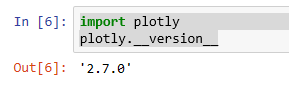
In this step, we’re checking for a package that is required to run our sample code. In the new field, enter the following and click the “Run” icon from the menu:

If you have the package, you should be seeing something like the following (the version can vary depending on the time of the installation):

If you see an error or a message indicating that you don’t have the package, use your Anaconda dashboard to install “plotly” for your Kernel. It’s a very intuitive process but is not covered in this document. The next step is to provide the “plotly” credential. For this step you normally have to have an account and a valid API key.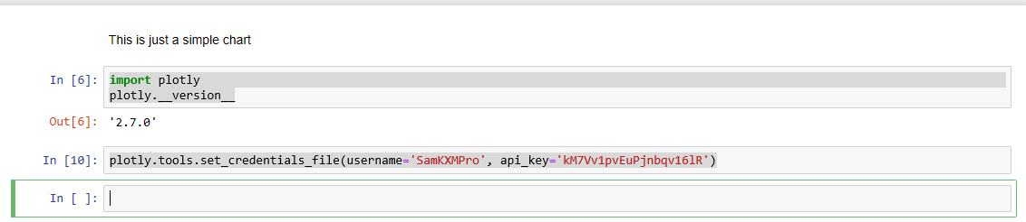

Running the cell will result in the credential being set and our use of the plotly authorized. It’s also a good time to mention that the cells that you run will retain their state in the Kernel, so in Cell 6 when we imported plotly it allowed us to then call set_credential_file in cell 10. You could go back and forth and modify the cells as you see fit in your own notebooks.

The next step is to create a simple Pie Chart, ensure that you have a Cell available and type the following in it:

 

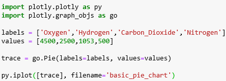
After you finish typing, run the application either by using the “Run” command in the menu or using the “CTRL+ “ENTER”.

The result will be the following Cell:

You could also try manipulating the values in the array and play around with them and then try running the cells again. As you can see use of Jupyter Notebook is quite intuitive and targets an audience that relies on rapid deployments of applications and information in general. The emphasis is more on visibility of ideas as data could easily be manipulated and results verified and/or proven.